Binomial Confidence Interval
and its application in reliability tests
(last updated on 2019-11-12)
Binomial confidence intervals are used when the data are dichotomous (e.g. 0 or
1, yes or no, success or failure). A binomial confidence interval provides an interval
of a certain outcome proportion (e.g. success rate) with a specified confidence level.
Reliability tests are in the category where binomial confidence intervals can be
applied. The outcome of each unit of a reliability test is either "success"
or "failure". A typical reliability test assesses a product's
reliability (i.e. success rate) for a specified duration. Each unit either
lasts for a specified duration or fails before the duration ends. For the failed
units, it does not consider when it fails. The test results are simply two numbers:
the sample size n and the number of successful units x. Based on these two numbers,
the reliability for any given confidence level, which is a one-sided confidence
interval, can be calculated.
There are two categories of methods to compute binomial confidence intervals -
approximation and exact. The approximations include
normal approximation,
Wilson score interval, Agresti-Coull interval, Jeffreys interval. The
exact methods are essentially variants the Clopper-Pearson interval. This note
focuses on the exact method because it provides us a window to look into the
real meaning and complexity
of confidence interval.
The word "exact" may give the impression that an exact method provide a crystal clear and simple understanding of how confidence
intervals are defined and computed. Crystal clear, maybe. Simple, probably
not. Thomas Ramsey, PhD provides
a succinct description of binomial confidence intervals with rigorous proof of the
equations for computing them. The 4-page paper may not be easily digestible
for most users of confidence intervals. Fortunately, users do not need to
understand the proof of the statistical equations applied in their work in most
cases. However, a good conceptual understanding is always beneficial. Dennis
P. Wash, PhD wrote an excellent
note on exact binomial confidence interval including an intuitive interpretation
and examples of computation. Jenő Reiczigel, PhD shows confidence interval
construction by test inversion in
a paper which
provides another perspective on how binomial confidence intervals are derived. David Harte, PhD has a
succinct and practical
note on how to compute the intervals using the F-distribution function and how
the method is derived.
The following is an effort to expand Wash's note
with the hope to help users of different backgrounds enhance their understanding
of the concept of confidence interval.
Suppose a study has n trials (e.g. n units under reliability test), x of the n trials
are successes (e.g. n - x units failed the test). The lower bound (pLB)
of the confidence interval (CI) with a confidence level of 100(1- α)% is obtained
by solving the following equation:
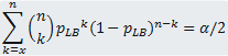 (Eq. 1)
The corresponding upper bound (pUB) is obtained by solving the following
equation:
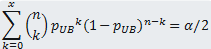 (Eq. 2)
Let us use an example to explain why the interval is determined by the above two
equations. Suppose there are 30 trials and 20 are successes, and the desired
confidence level is 90% (i.e. α = 0.05). The lower bound of the CI is the
lowest success probability that can be accepted with the current set of data.
Each success probability determines a binomial distribution (Fig. 1 shows two such
distributions). The distribution corresponding to pLB should
be such that the current data (i.e. 20 successes out of 30 trials) is barely rejected
with α = 0.05. In other words, the area of the upper tail starting at 20 (the
blue tail in Fig. 1 calculated with Eq. 1 ) equals 0.05. In this case, the distribution
with p = 0.05 meets the condition, so pLB = 0.50. Similarly, the upper
bound (pUB) should be the probability that is barely high enough to reject
20 with the significance level 0.05. In other words, the area of the lower
tail starting at 20 (the red tail in Fig. 1 calculated with Eq. 2) equals
0.05. In this case, the distribution with p = 0.81 meets the condition, so
pUB = 0.81. Please note the binomial distribution curves in Fig.
1 comprise discrete points each of which corresponds to an element of Eq. 1 or Eq.
2.
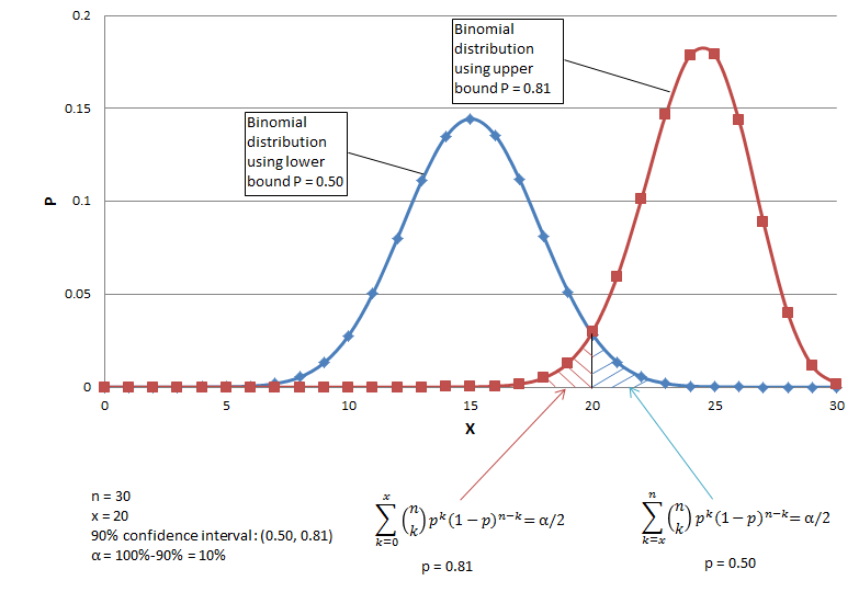
Fig. 1 An example of binomial trials and exact confidence interval
The above two equations can be directly used by a program to compute intervals
by solving them. A practical way of manually computing binomial confidence
intervals is using F-distribution functions. It is also a simple way to for
programs with access to an F-distribution function.
The lower bound:
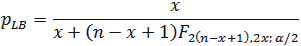 (eq. 3)
where F2(n-x+1),2x;α/2 is the F value with 2(n-x+1) numerator degrees
of freedom, 2x denominator degrees of freedom and the right tail area of α/2.
The upper bound:
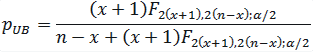 (eq.4)
where F2(x+1),2(n-x);α/2 is the F value with 2(x+1) numerator degrees
of freedom, 2(n-x) denominator degrees of freedom and the right tail area of
α/2.
For reliability tests, only the lower bound is concerned so α/2 should be
replaced with α in all the above equations. For example, to compute the lower bound for confidence level
90% (α = 0.1) using the F-distribution function, F2(n-x+1),2x;0.1 should be
used.
Related:
Binomial Confidence
Interval Calculator
Confidence Interval